

In situ cosmogenic isotopes are atoms that are formed directly within a particular material (such as rock or soil) on the Earth’s surface as a result of interactions with cosmic rays. Cosmic rays are high-energy particles from space, primarily protons, which collide with atoms in the Earth’s atmosphere and surface. These collisions can cause nuclear reactions that transform stable atoms within a mineral or rock into rare, radioactive isotopes, or cosmogenic isotopes.
The term “in situ” distinguishes these isotopes as being formed within the material itself, rather than being transported or deposited from elsewhere. These isotopes are valuable to scientists for a variety of reasons, especially in the fields of Earth science and geomorphology. By measuring the concentration of cosmogenic isotopes in surface rocks, researchers can estimate how long those surfaces have been exposed to the atmosphere, providing important insights into the timing of geological processes like erosion, sediment deposition, and the retreat of glaciers.
Commonly studied in situ cosmogenic isotopes include carbon-14 (^14C), beryllium-10 (^10Be), and aluminium-26 (^26Al). Each of these isotopes has a different half-life and production rate, making them useful for dating different time scales. For example, ^14C is used for relatively recent events (up to about 50,000 years ago), while ^10Be and ^26Al can be used to date geological surfaces that have been exposed for millions of years.
Al-26 meteorite exposure ages
Atmospheric production of 26Al is much lower than 14C or 10Be because the progenitor, 40Ar, constitutes only about 1% of atmospheric gases. In situ production at the Earth’s surface is also low, due to atmospheric attenuation of cosmic rays. Consequently, the first measurements of cosmogenic 26Al were in studies of the Moon and meteorites. After the break-up of their parent bodies, meteorite fragments are exposed to intense cosmic-ray bombardment during their travel through space, causing substantial 26Al production. If these fragments have cosmic exposure ages of at least a few Myr, their surfaces will reach saturation in 26Al (t1/2 = 0.7 Myr).
After falling to Earth, atmospheric shielding protects meteorite fragments from significant further 26Al production, and decay of this inventory can then be used to determine a terrestrial residence age. Because the abundances of 26Al in meteorites are comparatively high they do not demand accelerator mass spectrometry. Instead, they are measured using non-destructive ( counting, by putting the whole meteorite fragment in a large shielded detector. Attenuation of ( particles by the sample itself is corrected by empirical modelling (e.g. Evans et al., 1979).
In the first large-scale survey of Antarctic meteorites, Evans et al. (1979) compared the 26Al activities in these samples with those in ‘falls’ (observed at impact), which have a zero terrestrial residence. The falls had a moderately well-defined range of 26Al activities for a given compositional class of meteorites (Fig. 14.48). The outlier from this class can be attributed to a failure to reach 26Al saturation, due to the short cosmic-ray exposure history of the fragment. In contrast, Antarctic meteorites ranged to substantially lower activities, indicating significant terrestrial residence ages in several cases. Unfortunately, these values are only semi-quantitative, due the relatively long half-life of 26Al, and due to uncertainties in production. The latter problem arises because of the poor penetrative capacity of the low-energy cosmic rays which generate 26Al, making the cosmic production rate susceptible to depth within the fragment.
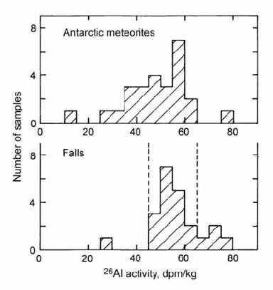
Fig. 14.48. Histogram of 26Al activities in Antarctic meteorites, compared with American ‘falls’. After Evans et al. (1979).
Although 26Al represents a good reconnaissance tool for terrestrial age determination (e.g. Evans and Reeves, 1987), 36Cl provides a more precise method (Nishiizumi et al., 1979). This arises from its shorter (0.3 Myr) half-life, and from more accurately known saturation values, due to its generation by penetrative high-energy cosmic rays. However, the analysis is more technically demanding, and must be performed by accelerator mass spectrometry. Results of a large 36Cl study of Antarctic meteorite ages are shown in Fig. 14.49 (Nishiizumi et al., 1989a).
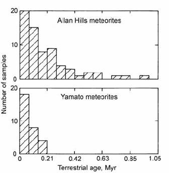
Fig. 14.49. Histograms of calculated terrestrial residence age for Antarctic meteorites from the Allan Hills and Yamato Mountains areas, based on the decay of cosmogenic 36Cl. After Nishiizumi et al. (1989a).
The high quality of terrestrial 36Cl ages for Antarctic meteorites has led to their use to determine the half-life of another cosmogenic nuclide, 41Ca. With a half-life of only 0.1 Myr, this shows promise as a precise dating tool, but an efficient AMS analysis method has only recently been developed (Fink et al. 1990). Another problem limiting the application of 41Ca has been uncertainty in the half-life. To solve this problem, Klein et al. (1991) performed 41Ca analyses on aliquots of Antarctic iron meteorites which had already been dated by 36Cl. The results revealed a strong linear correlation between the abundance of the two species, whose slope corresponds to the ratio of the half-lives. Taking a 36Cl half-life of 301 ” 4 kyr yields a precise 41Ca half-life of 103 ” 7 kyr.
14.6.2 Al–Be terrestrial exposure ages
Because of atmospheric attenuation of cosmic rays, most terrestrial materials have 26Al/27Al ratios less than 10!14. However, in some aluminium-poor minerals such a quartz, the content of (non-cosmogenic) 27Al may be as low as few ppm, so that after a few thousand years of exposure to cosmic rays, 26Al/27Al ratios of 10!11 to 10!13 may be generated, within the measurement range of AMS. These data can then be used to calculate exposure ages of terrestrial rock surfaces.
The principal obstacle to AMS analysis of 26Al is the formation of sufficient negative Al ions during sputtering, which is only about 25% efficient (Middleton and Klein, 1987). The metal species must be used rather than the oxide because the latter suffers a severe interference from MgO. However, Mg does not form negative metal ions at all, so there are no isobaric interferences on the Al metal-ion signal.
The principal application of 26Al as a geochronometer is in the measurement of rock exposure ages. It would be possible to use this nuclide alone for this purpose, but in view of the many possible permutations of exposure and erosion history, the use of two nuclides with different half-lives provides a more powerful constraint on these models. The normal choice is to combine 26Al measurements (t1/2 = 0.705 Myr) with 10Be (t1/2 = 1.51 Myr).
The atmospheric 26Al/10Be production ratio has been determined as about 4 H 10!3 by sampling from high-flying aircraft, but the in situ production ratio in quartz has been measured as 6 (Nishiizumi et al., 1989b). Because the atmospheric 10Be production rate is comparatively high, great care must be taken to ensure that rock samples to be used for exposure dating are not contaminated by the atmospheric or so-called ‘garden variety’ of 10Be (Nishiizumi et al., 1986). Because of its resistance to chemical weathering, quartz is comparatively resistant to contamination by ‘garden variety’ 10Be. This, along with its low 27Al content makes it an excellent material for exposure dating. In quartz, 10Be is derived from spallation of 16O, while 26Al is produced by spallation of 28Si and mu-meson capture by the same species. Most of this production occurs in the top half-metre of the rock surface, but limited 26Al production can occur at depths of up to 10 m (Middleton and Klein, 1987).
Interpretations of Surface Exposure Data
There are two limiting models for the interpretation of surface exposure data (e.g. Nishiizumi et al., 1991a). These are illustrated on a plot of 26Al/10Be ratio against absolute 10Be abundance (Fig. 14.50). The upper curve shows the effect of increasing exposure age, for the case where the erosion rate is zero. The lower curve shows the effect of different steady-state erosion rates, for the case where exposure age is infinite (relative to the half-lives of 26Al and 10Be). At the point of saturation (after a few half-lives), the 26Al/10Be ratio is 2.88. Unfortunately, the limited (factor of two) difference between the half-lives of 26Al and 10Be causes only a relatively small separation between the curves for the two end-member models. This places limits on the resolving power of the Al–Be method, given the relatively large analytical errors on the AMS measurements.
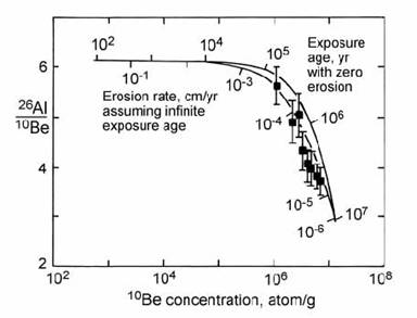
Fig. 14.50. Plot of analysed 26Al/10Be against 10Be abundance (corrected to production at sea-level) for Allan Hills quartz samples, used as a measure of minimum exposure age and/or maximum erosion rate. After Nishiizumi et al. (1991a).
Application of the Al)Be exposure method is demonstrated in Fig. 14.50 using data from nunataks of the Allan Hills area of Antarctica (Nishiizumi et al., 1991a). The results display a range of Al/Be ratios close to the steady-state erosion curve. However, the zero-erosion-rate (variable exposure age) model cannot be ruled out. The lowest 26Al/10Be yields the strongest constraint, representing a minimum exposure age of 1.4 Myr or a maximum erosion rate of 0.24 mm/kyr. Samples to the left of the erosion line in Fig. 14.50 may be explained by burial under ice for some period in the past. During times of burial, points move downwards to the left, due to the greater rate of decay of 26Al relative to 10Be.
The combination of these two cosmogenic isotopes can also be used to date sediment burial, as demonstrated by Granger et al. (2001) in a dating study on cave sediments from Mammoth Cave, Kentucky. Sediments entered this cave system from the Green River, a tributary of the Ohio River, which cut down into a karst landscape. There is a very strong likelihood that sediments were exposed on the land surface prior to their transport and deposition in the cave system. Therefore, quartz grains in the sediment are expected to have reached steady state abundances of cosmogenic Al and Be, with a 26Al/10Be saturation ratio of 6 (Fig. 14.51).
After burial in the cave system, radioactive decay begins, and the samples follow a trend to the lower left in Fig. 14.51. This allows the dating of sediments at different levels in the cave system, so that the down-cutting of the river can be traced against time. Projection of the decay trend back to the steady state line also allows the erosion rate of the surficial sediment source to be estimated at around 3 m / Myr. The combination of 26Al and 10Be is particularly suitable for burial dating because the pre-burial cosmogenic production of the two nuclides occurs under similar conditions. Accurate modelling of isotope production during the surface exposure history of the sediment is a prerequisite to obtaining accurate burial ages (Granger and Muzikar, 2001).
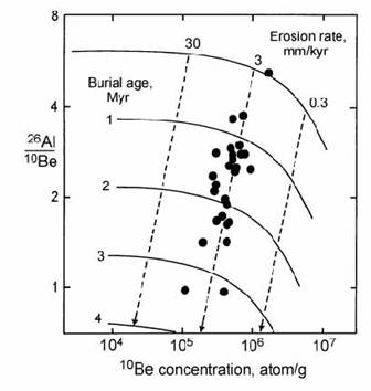
Fig. 14.51. Plot of analysed 26Al/10Be against 10Be in sediments from different levels in Mammoth Cave, Kentucky. Vertical displacements allow the dating of cave deposits from their burial ages, while the intersection with the exposure curve indicates an erosion rate of 3 mm/kyr for the sediment source. After Granger et al. (2001).
Chlorine-36 Exposure Ages
The concept of exposure dating using in situ produced cosmogenic 36Cl was suggested by Davis and Schaeffer (1955), but could not be effectively applied until the advent of AMS analysis (Phillips et al., 1986). Although developed after the 10Be and 26Al methods, 36Cl offers several advantages. It is applicable to a variety of rock types because it is generated from three parents (K, Ca, and Cl) with different chemistry, while most rocks have low background levels of chlorine. Furthermore, interferences by nucleogenic 36Cl are minimal, and contamination from atmospheric 36Cl is only a problem in severely weathered material.
The three main sources of in situ cosmogenic 36Cl are neutron activation of 35Cl and neutron-induced spallation of 40K and 40Ca. A subordinate source is from negative muon capture by 40Ca. The relative importance of these production routes depends on the relative K: Ca: Cl abundances in the target and the degree of shielding by overlying rock. Zreda et al. (1991) made an empirical study of spallation production, while Liu et al. (1994) studied the depth dependence of the neutron activation reaction. Spallation reactions are caused by fast neutrons, which decrease exponentially with depth. However, activation reactions require (slow) thermal neutrons, which are produced when fast neutrons undergo glancing collisions with substrate atoms. Hence, slow neutrons reach a peak intensity at about 15 cm depth in rocks (Fig. 14.52). The occurrence of multiple routes makes the calculation of total production rates more complex, but it also offers the possibility of greater age control, as will be shown below.
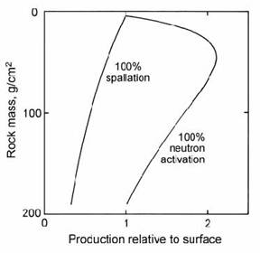
Fig. 14.52. Calculated production profiles for 36Cl by spallation and neutron activation (normalised to equal values at the surface) as a function of rock mass per unit area. After Liu et al. (1994).
The simplest scenario for cosmogenic dating is the instantaneous transport of rock from below the cosmic-ray penetration depth to the surface, followed by exposure without shielding by other material (such as snow cover) and without significant erosion. In this case, all production routes for 36Cl can be summed. However, corrections must be made for the latitude dependence of cosmic-ray intensity and the altitude dependence of atmospheric shielding.
A relatively simple scenario is provided by surface-exposure dating of rocks at Meteor Crater, Arizona (Nishiizumi et al., 1991b). Samples were taken from the upper few cm of large blocks in the ejecta blanket of the impact. The lithology of these blocks shows that they were from strata buried at depths of over 10 m before the impact. On the other hand, their large size suggests that they were unroofed of any overlying ash blanket soon after the impact event. The surfaces of the sampled ejecta blocks were found to be coated with ‘rock varnish’, which takes thousands of years to develop. Therefore, erosion was probably negligible in the arid climate of Arizona, so that 36Cl abundances translate directly into an exposure age. A good agreement was reached between 36Cl and Al–Be ages, with a consensus of ages around 50 kyr. A few younger ages (e.g., Monument Rock) may indicate more recent exposure of these blocks above the ash blanket.
Another type of simple scenario is achieved in relatively young lava flows, which are instantaneously exposed at the surface and have not yet suffered significant weathering. However, in many geological environments, erosion is a significant factor. In this case, a single cosmogenic isotope determination only allows the solution of exposure age at a known erosion rate or erosion rate at a known exposure age. For example, using a lava flow from Nevada of known age, Shepard et al. (1995) were able to estimate the weathering rate based on 36Cl/35Cl ratios.
A more complex scenario arises when both the exposure age and the erosion rate of a deposit are unknown. This applies particularly to rapidly eroding sedimentary deposits. To investigate the constraints which may be applied to such a system, Zreda et al. (1994) considered a theoretical model for the erosional exposure of a deposit with buried clasts. These clasts, initially buried within the deposit, are gradually exposed at the surface by erosion of the fine- grained matrix (Fig. 14.53). This model applies to the problem of dating glacial moraines based on the exposure ages of boulders on the moraine surface, and also to dating meteorite impacts based on blocks exposed on the ejecta blanket. Zreda et al. argued that if 36Cl dates are available from several different boulders on a moraine or ejecta blanket, the spread of ages (outside analytical error) could be used to model the exposure history of the deposit.
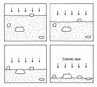
Fig. 14.53. Schematic illustration of the exhumation of clasts from a heterogeneous deposit by erosion of the matrix. After Zreda et al. (1994).
To demonstrate these effects, Zreda and Phillips (1995) modelled 36Cl/Cl ratios for several boulders buried at depths from zero to 300 g/cm2 (approximately 1.5 m depth in soil of density equal to 2). Total 36Cl production was attributed 50% to spallation reactions and 50% to neutron activation. The erosion rate was set so that the deepest boulder just reaches the surface at the present day. The modelling results show a wide range of 36Cl/Cl ratios, both below and slightly above the growth curve for zero depth (Fig 14.54). The growth curves for deeply buried boulders start with slow production, due to the shielding effect of the overlying matrix. As the boulder approaches the surface, the rate of production accelerates, but the total 36Cl inventory remains well below that of a surface sample. On the other hand, boulders which were initially subject to shallow burial can actually show greater total 36Cl production than at the surface, due to the peak of neutron activation production at a depth of 50 g/cm2.
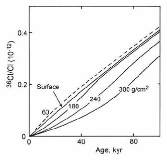
Fig. 14.54. Modeled 36Cl/Cl inventories for rock boulders buried at various depths in an eroding deposit, showing peak cosmogenic production just below the surface. After Zreda and Phillips (1995).
Zreda and Phillips (1995) modeled the erosion history of ejecta blocks from Meteor Crater, Arizona, in a similar way. However, in this case the spread of apparent exposure ages was based on 1000 model points randomly buried from zero to a chosen maximum depth (Fig. 14.55). The model results were compared with the actual spread of ages in four blocks at Meteor Crater, with a mean age of 49.7 ” 0.9 kyr (Monument Rock was excluded). The best fit was obtained by assuming burial to a maximum depth of 300 g/cm2 (ca. 1.5 m), removed at 30 g/cm2/kyr (0.15 mm/yr), so that all boulders reached the surface within 10 kyr. Such modeling cannot yield a unique solution to the erosion process, and the model results should ideally be compared with a larger set of measured ages. Nevertheless, the modeling does suggest that the four blocks yield exposure ages close to the estimated time of impact.
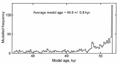
Fig. 14.55. Histogram of model 36Cl exposure ages for 1000 rock clasts exhumed from depths up to ca. 1.5 m in a deposit with a formation age of 50 kyr. A few samples overestimate the real age due to greater cosmogenic production just below the surface. After Zreda and Phillips (1995).
In principle, the use of two spallogenic nuclides (e.g., 10Be and 26Al) allows the deconvolution of exposure ages and erosion rates. However, as noted above, the closely spaced trajectories of the constant erosion and the constant exposure saturation lines make the deconvolution weak (e.g. Fig. 14.39). A more powerful application of the 36Cl technique makes use of the neutron activation route to 36Cl, in comparison with the pure spallation nuclides (10Be or 26Al). Because spallation and neutron activation yield peak nuclide production at different depths in a geological surface, they should yield a clear resolution of exposure histories involving different rates of erosion (Liu et al., 1994). With this objective in mind, Bierman et al. (1995) described a method for isolating the neutron activation component of 36Cl, by releasing chlorine from fluid inclusions within rock samples. However, the method has not been demonstrated in practice. Alternatively, a crude assessment of the rate of erosion can be obtained by simply ignoring spallogenic 36Cl production.
This approach was taken by Phillips et al. (1997) in a study on glacial deposits of the Wind River Range, Wyoming. Ten boulders from glacial moraines were analyzed for both 36Cl and 10Be, and are plotted on the Cl–Be plot in Fig. 14.56. The limits for zero erosion and for infinite age (erosional equilibrium) are given, as in the Al–Be plot. However, they are now much further apart, allowing easy resolution between the two models. Most of the data lie below the line corresponding to 0.5 mm of erosion per kyr, indicating that the surfaces of these boulders are not undergoing significant loss by erosion. The boulders were sampled from six different moraines, and their ages indicate that one moraine dates from the last glaciation (ca. 20 kyr), three from the penultimate glaciation (ca. 130 –100 kyr) and two from older glaciations, assuming rapid exposure of the boulders on the moraine surface.

Fig. 14.56. The plot of analyzed 36Cl/10Be against 36Cl abundance for boulders from glacial moraines of the Wind River Range, Wyoming. Solid lines indicate erosion rates; dashed lines are exposure-age isochrons. See text for discussion. After Phillips et al. (1997).
A different application of the 36Cl method was proposed by Stone et al. (1996), using 40Ca spallation as a tool for exposure dating of calcite. The abundance of the target nuclide, along with the relatively low abundance of chlorine in calcite, makes this an analytically favorable method that shows great promise for exposure dating of karst landscapes. For example, two recent studies (Zreda and Noller, 1998; Mitchell et al., 2001) used 36Cl abundances in fault scarps to date the displacement of fault systems in carbonate rocks. In both cases, 36Cl measurements were made at several points down the face of the fault scarp. 36Cl accumulation was then used to determine the date when each sample was first exposed at the surface, allowing a reconstruction of past movement on the fault.
The Relationship Between Cosmogenic Isotopes and Allergy Studies
Cosmogenic isotopes, while primarily known for their applications in geosciences and climatology, also intersect with medical and health-related fields, including the study of allergies. This connection, though not immediately obvious, can be understood through the broader implications of environmental changes on human health.
Cosmogenic isotopes, such as beryllium-10 (^10Be) and carbon-14 (^14C), are produced by the interaction of cosmic rays with the Earth’s atmosphere and surface materials. These isotopes are used by scientists to understand various aspects of the Earth’s environmental history, including climate change, erosion rates, and the exposure age of surfaces. The production rates of these isotopes can be influenced by solar activity and Earth’s magnetic field, both of which modulate the flux of cosmic rays reaching the Earth.
The connection to allergies comes through the environmental changes these isotopes help to reconstruct. For instance, climate change, evidenced by variations in cosmogenic isotope concentrations, can lead to shifts in plant blooming times, the distribution of allergenic plant species, and the concentration of pollen in the air. These changes can have direct impacts on allergy prevalence and severity among the human population.
Increased temperatures and CO2 concentrations can lead to longer pollen seasons and higher pollen counts, exacerbating allergic reactions. Additionally, changes in precipitation patterns and humidity, also related to climate change, can affect mold spore levels, another common allergen. By studying cosmogenic isotopes, scientists can gain insights into past climate conditions and predict future trends, indirectly informing us about potential changes in allergy patterns.
Furthermore, understanding the environmental and climatic conditions that favor the proliferation of certain plants or molds can help develop mitigation strategies for allergies. For example, urban planning and landscaping can consider the types of vegetation that are less likely to exacerbate allergies.
Human activities and mobility, influenced by climatic and environmental changes, also play a crucial role in the spread of allergens. Changes in land use, agriculture, and urbanization, driven by environmental conditions that are traced through cosmogenic isotope studies, can introduce or eliminate habitats for various plant and animal species that are sources of allergens. Understanding these dynamics is crucial for developing strategies to manage and reduce the impact of allergens on public health.
In summary, the study of in situ cosmogenic isotopes offers valuable insights into environmental changes that, in turn, can impact allergy trends. By bridging the gap between geosciences and medical research, we can better understand the complex interactions between our planet’s climate system and human health, potentially leading to more effective allergy prevention and management strategies.
REFERENCES
Adkins, J. F. and Boyle, E. A. (1997). Changing atmospheric ) 14C and the record of deep water paleoventilation ages. Paleoceanography 12, 337–44.
Anderson, E. C. and Libby, W. F. (1951). World-wide distribution of natural radiocarbon. Phys. Rev. 81, 64)9.
Andree, M., Oeschger, H., Broecker, W., Beaven, N., Klas, M., Bonani, G., Hoffman, H. J., Suter, M., Woelfli, W. and Peng, T.-H. (1986). Limits on ventilation rates for the deep ocean over the last 12,000 years. Climate Dynamics 1, 53–62.
Andrews, J. N., Davis, S. N., Fabryka-Martin, J., Fontes, J. C., Lehmann, B. E., Loosli, H. H., Michelot, J-L., Moser, H., Smith, B. and Wolf, M. (1989). The in situ production of radioisotopes in rock matrices with particular reference to the Stripa granite. Geochim. Cosmochim. Acta 53, 1803)15.
Arnold, J. R. (1956). Beryllium-10 produced by cosmic rays. Science 124, 584)5.
Arnold, J. R. (1958). Trace elements and transport rates in the ocean. 2nd UN Conf. on Peaceful Uses of Atomic Energy 18, 344)6. IAEA.
Arnold, J. R. and Libby, W. F. (1949). Age determinations by radiocarbon content: Checks with samples of known age. Science 110, 678)80.
Bard, E., Arnold, M., Fairbanks, R. G. and Hamelin, B. (1993). 230Th)234U and 14C ages obtained by mass spectrometry on corals. Radiocarbon 35, 191)9.
Bard, E., Arnold, M., Hamelin, B., Tisnerat-Laborde, N. and Cabioch, G. (1998). Radiocarbon calibration by means of mass spectrometric 230Th/234U and 14C ages of corals: an updated database including samples from Barbados, Mururoa and Tahiti. Radiocarbon 40, 1085–92.
Bard, E., Arnold, M., Mangerud, J., Paterne, M., Labeyrie, L., Duprat, J., Melieres, M. A., Sonstegaard, E. and Duplessy, J. C. (1994). The North Atlantic atmosphere–sea surface 14C gradient during the Younger Dryas climatic event. Earth Planet. Sci. Lett. 126, 275–87.
Bard, E., Hamelin, B., Fairbanks, R. G. and Zindler, A. (1990a). Calibration of the 14C timescale over the past 30,000 years using mass spectrometric U)Th ages from Barbados corals. Nature 345, 405)10.
Bard, E., Hamelin, B., Fairbanks, R. G., Zindler, A., Mathieu, G. and Arnold, M. (1990b). U/Th and 14C ages of corals from Barbados and their use for calibrating the 14C timescale beyond 9000 years B.P. Nucl. Instr. Meth. in Phys. Res. B 52, 461)8.
Bard, E., Raisbeck, G. M., Yiou, F. and Jouzel, J. (1997). Solar modulation of cosmogenic nuclide production over the last millennium: comparison between 14C and 10Be records. Earth Planet. Sci. Lett. 150, 453–62.
Baumgartner, S., Beer, J., Masarik, J., Wagner, G., Meynadier, L. and Synal, H.-A. (1998). Geomagnetic modulation of the 36Cl flux in the GRIP ice core, Greenland. Science 279, 1330–32.
Baxter, M. S. and Farmer, J. G. (1973). Radiocarbon: short-term variations. Earth Planet. Sci. Lett. 20, 295)9.
Beck, J. W., Richards, D. A., Edwards, R. L., Silverman, B. W., Smart, P. L., Donahue, D. J., Hererra-Osterheld, S., Burr, G. S., Calsoyas, L., Jull, A. J. T. and Biddulph, D. (2001). Extremely large variations of atmospheric 14C concentration during the last glacial period. Science 292, 2453–8.
Beer, J., Andree, M., Oeschger, H., Siegenthaler, U., Bonani, G., Hofmann, H., Morenzoni, E., Nessi, M., Suter, M., Wolfli, W., Finkel, R. and Langway, C. (1984). The Camp Century 10Be record: implications for long-term variations of the geomagnetic dipole moment. Nucl. Instr. Meth. in Phys. Res. B 5, 380)4.
Beer, J., Oeschger, H., Finkel, R. C., Castagnoli, G., Bonino, G., Attolini, M. R. and Galli, M. (1985). Accelerator measurements of 10Be: the 11 year solar cycle. Nucl. Instr. Meth. in Phys. Res. B 10, 415)18.
Beer, J., Siegenthaler, U., Bonani, G., Finkel, R. C., Oeschger, H., Suter, M. and Wolfli, W. (1988). Information on past solar activity and geomagnetism from 10Be in the Camp Century ice core. Nature 331, 675)9.
Belshaw, N. S., O’Nions, R.K., and von Blankenburg, F. (1995). A SIMS method for 10Be/9Be ratio measurement in environmental materials. Int. J. Mass Spectrom. Ion Phys. 142, 55–67.
Bentley, H. W., Phillips, F. M., Davis, S. N., Gifford, S., Elmore, D., Tubbs, L. E. and Gove, H. E. (1982). Thermonuclear 36Cl pulse in natural water. Nature 300, 737)40.
Bentley, H. W., Phillips, F. M., Davis, S. N., Habermehl, M. A., Airey, P. L., Calf, G. E., Elmore, D., Gove, H. E. and Torgerson, T. (1986). Chlorine 36 dating of very old groundwaters, 1, The Great Artesian Basin, Australia. Water Resour. Res. 22, 1991)2002.
Bierman, P., Gillespie, A., Caffee, M. and Elmore, D. (1995). Estimating erosion rates and exposure ages with 36Cl produced by neutron activation. Geochim. Cosmochim. Acta 59, 3779–98.
Broecker, W. S. and Denton, G. H. (1989). The role of ocean–atmosphere reorganizations in glacial cycles. Geochim. Cosmochim. Acta 53, 2465–2501.
Broecker, W. S., Gerard, R., Ewing, M. and Heezen, B. C. (1960). Natural radiocarbon in the Atlantic Ocean. J. Geophys. Res. 65, 2903–31.
Brown, E. T., Edmond, J. M., Raisbeck, G. M., Bourles, D. L., Yiou, F. and Measures, C. I. (1992). Beryllium isotope geochemistry in tropical basins. Geochim. Cosmochim. Acta 56, 1607)1624.
Brown, L., Klein, J. and Middleton, R. (1985). Anomalous isotopic concentrations in the sea off Southern California. Geochim. Cosmochim. Acta 49, 153)7.
Brown, L., Klein, J., Middleton, R., Sacks, I. S. and Tera, F. (1982). 10Be in island-arc volcanoes and implications for subduction. Nature 299, 718)20.
Brown, L., Stensland, G. J., Klein, J. and Middleton, R. (1989). Atmospheric deposition of 7Be and 10Be. Geochim. Cosmochim. Acta 53, 135)42.
Bruns, M., Rhein, M., Linick, T. W. and Suess, H. E. (1983). The atmospheric 14C level in the 7th millennium BC. P.A.C.T. (Physical And Chemical Techniques in Archaeology) 8, 511)6.
Bucha, V. and Neustupny, E. (1967). Changes in the Earth’s magnetic field and radiocarbon dating. Nature 215, 261)3.
Campin, J.-M., Fichefet, T. and Duplessy, J.-C. (1999). Problems with using radiocarbon to infer ocean ventilation rates for past and present climates. Earth Planet. Sci. Lett. 165, 17–24.
Chengde, S., Beer, J., Tungsheng, L., Oeschger, H., Bonani, G., Suter, M. and Wolfli, W. (1992). 10Be in Chinese loess. Earth Planet. Sci. Lett. 109, 169)77.